
USE Text Embeddings, vector similarities for text classification and their equivalences.
One way of classifying texts into categories is to assign to a new given text the category of the most similar text in the training set. Given vector representations of the texts, there are many similarity metrics that can be chosen, however, some of them can yield the exact same accuracy.
10kGNAD is a topic classification dataset/task consisting of German news articles and their corresponding topics (Economy, Politics, Sport, etc). As defined, the training set has a total of 9245 articles divided into 9 categories and the test set is composed by 1028 articles divided in the same categories.
One way of tackling this task is:
- Compute vector representations of the training dataset articles.
- Given a test article, compute its vector representation.
- Calculate the similarity between the test article and every article in the training dataset.
- Assign to the test article the category of the most similar article.
Universal Sentence Encoder (USE): Multilingual Version
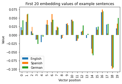
For computing the text embeddings (see HERE if you want to know more about this topic), we can use a pretrained model made publicly available by Google: the Universal Sentence Encoder, USE. In its multilingual version, this model computes text embeddings which will be similar for texts that are semantically similar even if they are not in the same language. For example:
df = pd.DataFrame()
df["English"] = embed("I am Héctor and work as a Data Scientist")[0]
df["Spanish"] = embed("Soy Héctor y trabajo de científico de datos")[0]
df["German"] = embed("Ich bin Héctor und arbeite als Datenwissenschaftler")[0]

df.iloc[:20].plot(kind="bar")
As we can see in the plot below, those positions in the embeddings that are large for one language are also large for the other two languages. The correlations among these embeddings are higher than 0.9.
Using USE in Google Colab
For using USE in Google Colab, we only have to install tensorflow-text by doing:
!pip install -q tensorflow-text
Then we can access the model’s API by doing:
import tensorflow_hub as hub
import tensorflow_text

embed = hub.load("https://tfhub.dev/google/universal-sentence-encoder-multilingual-large/3")
and then we are ready.
The task
If you want, you can follow along the post with this Google Colab where the code has been implemented.
First, we need to download the dataset following the instructions in the GitHub repository or by curl-ing it:
!wget https://raw.githubusercontent.com/tblock/10kGNAD/master/train.csv
!wget https://raw.githubusercontent.com/tblock/10kGNAD/master/test.csv
Then, I read the training and test datasets into a Pandas Dataframe (Side note: I don’t use the
Pandas read_csv as some of the texts also contain the separators).
def read_dataset_into_pandas_csv(path):

  all_rows = []
  with open(path, mode="r") as f:
    for row in f.readlines():
      all_rows.append(row.split(";", 1))

  df = pd.DataFrame(data=all_rows, columns=["category", "text"])
  return df

train_df = read_dataset_into_pandas_csv("train.csv")
test_df = read_dataset_into_pandas_csv("test.csv")
To reduce the computational complexity of the task, I will only use 5 articles per topic in the training set and 10 per topic in the test dataset.
def select_n_articles_per_category(dataset, n_articles_per_category):
  X = []
  Y = []

  for category, category_rows in dataset.groupby("category"):
    Y.extend(category_rows.category.iloc[:n_articles_per_category])
    X.extend(category_rows.text.iloc[:n_articles_per_category])

  return X, Y

X_train, Y_train = select_n_articles_per_category(train_df, 5)
X_test, Y_test = select_n_articles_per_category(test_df, 10)
Then, I obtain the embeddings version of the article texts:
X_train = [embed(x)[0] for x in tqdm(X_train)]
X_test = [embed(x)[0] for x in tqdm(X_test)]
One way of predicting is to compute pairwise similarities between the test articles
and the training articles and choose the most similar article’s class as the answer.
One example of a similarity metric is cosine_similarity, which comes implemented in scikit-learn:
from sklearn.metrics.pairwise import cosine_similarity

similarities = cosine_similarity(X_test, X_train) #shape: (#Test articles, #Train articles)
most_similar_articles = np.argmax(similarities, axis=1) # shape (#Test articles)
Then we obtain the classes that correspond to the most similar articles and check our accuracy:
most_similar_articles_classes = [Y_train[i] for i in most_similar_articles]
accuracy = np.mean(np.array(most_similar_articles_classes) == np.array(Y_test))
This approach obtains a 53.33% accuracy (random accuracy = 1/9 = 11.11%), which is not bad given that we haven’t had to train any additional model and we are using only 5 articles per topic as a training set.
Alternatives to cosine similarity
There are many alternatives to cosine similarity. To name a few similarity/distance metrics:
# Distance metrics
Manhattan distance (A, B) = |a_1 - b_1| + |a_2 - b_2| + ... + |a_n - b_n| = ||A-B||_1
Euclidean distance (A, B) = sqrt((a_1 - b_1)^2 + (a_2 - b_2)^2 + ... + (a_n - b_n)^2)
                          = sqrt( <A, B> x <A, B> ) =  ||A - B||

# Similarity metrics / kernels
Cosine similarity (A, B) = <A, B> / ( ||A|| ||B|| )
Linear kernel (A, B) = <A, B>
RBF kernel (A, B) = exp(-gamma ||A - B||^2)
Pearson correlation
Spearman's Rank correlation
where <A, B> refers to the inner product between A and B (A^T B), ||X|| refers to the 2-norm of X and ||X||_1 to the 1-norm of X.
One way of transforming a distance metric D into a similarity metric is to inverse it as follows:
S(A, B) = exp(-D(A, B) x gamma) # where gamma is a chosen constant

# Manhattan similarity = exp(-gamma ||A - B||_1)
# Euclidean similarity = exp(-gamma ||A - B||)
Note: The similarity equivalent of the Manhattan distance is also referred to as Laplacian kernel.
Calculating the accuracy for the alternatives
To define the distances and correlation metrics as a pairwise metric usable in the same way scikit-learn does, we can do:
manhattan_similarity = lambda X, Y: np.exp(-manhattan_distances(X, Y))
euclidean_similarity = lambda X, Y: np.exp(-euclidean_distances(X, Y))
pearson_correlation = lambda X, Y: [[np.corrcoef(x, y)[0][1] for y in Y] for x in X]
spearman_correlation = lambda X, Y: [[spearmanr(x, y)[0] for y in Y] for x in X]
Then, we can simply plug in the chosen similarity metric in the same way as before:
def get_accuracy_for_similarity_metric(similarity_metric):
  similarities = similarity_metric(X_test, X_train)
  most_similar_articles = np.argmax(similarities, axis=1)
  most_similar_articles_classes = [Y_train[i] for i in most_similar_articles]
  return np.mean(np.array(most_similar_articles_classes) == np.array(Y_test))
With this, we can run a comparison among metrics:
labels = ["Manhattan Similarity", "Euclidean Similarity", "Linear Kernel", "Cosine Similarity",
          "RBF Kernel", "Pearson Correlation", "Spearman's Rank Correlation"]
metrics = [manhattan_similarity, euclidean_similarity, linear_kernel, cosine_similarity,
           rbf_kernel, pearson_correlation, spearman_correlation]

for label, similarity_metric in zip(labels, metrics):
  accuracy = get_accuracy_for_similarity_metric(similarity_metric)
  print("%s: %.2f%%" % (label, accuracy * 100))
Accuracy of each of the metrics:
Manhattan Similarity: 55.56%
Euclidean Similarity: 53.33%
Linear Kernel: 53.33%
Cosine Similarity: 53.33%
RBF Kernel: 53.33%
Pearson Correlation: 52.22%
Spearman's Rank Correlation: 54.44%
Manhattan Similarity (aka Laplacian Kernel) seems to work marginally better in this reduced dataset. However, more surprisingly:
4/7 metrics tested (Euclidean, Linear Kernel, Cosine Similarity and RBF Kernel) have the exact same accuracy. Why is this? Well, math.
Equivalence / proportionality between similarity metrics
In one way or another, these apparently different metrics are equivalent to each other.
Let’s start off with Linear Kernel and Cosine similarity. A Linear Kernel is simply the inner product between two vectors. The cosine similarity, is a normalised version of this product. Where is the trick here? The output of the Universal Sentence Encoder is L2-normalised, which means that ||A|| = ||B|| = 1, rendering Linear Kernel and Cosine similarity the exact same:
Linear kernel (A, B) = <A, B>
Cosine similarity (A, B) = <A, B> / ( ||A|| ||B|| ) = <A, B> / (1 x 1) = <A, B> = Linear Kernel
For the remaining comparisons, we have to take into account an important fact:
If two metrics are a monotonic increasing function of each other, they will have the same accuracy since the ordering won’t vary across them.
An easy way of seeing this is by thinking about finding the index of the largest item in a list:
[30, 7, 6, 4] # the 1st item is the largest
and the largest item in the same list where every element is multiplied by 3
[90, 21, 18, 12] # The 1st item is still the largest item
In this toy example “multiplying by 3” is a monotonic function as it preserves the order of the elements in the list.
How is this reflected in the other metrics shown? Well, the RBF kernel can be seen as a version of the euclidean similarity, where the Euclidean distance appears squared:
Euclidean similarity (A, B) = exp(-gamma ||A - B||)
RBF kernel (A, B) = exp(-gamma ||A - B||^2)
Since squaring is an increasingly monotonic function, the ordering of elements will be preserved and the accuracy of both methods will remain the same.
Lastly, Euclidean distance and Cosine Similarity are related as follows:
Cosine similarity (A, B) = <A, B> / ( ||A|| ||B|| ) = <A, B> / (1 x 1) = <A, B>
Euclidean distance (A, B) = sqrt( (A - B)^T (A - B) ) = sqrt ( A^T A - A^T B - B^T A + B^T B ) =
                          = sqrt( 1 - 2 * A^T B + 1 ) = sqrt( 2 - 2 A^T B ) = sqrt( 2 - 2 Cosine similarity (A, B) )
The higher the cosine similarity between A, B (up to 1), the lower the distance will be. The smaller the similarity between A, B (up to 0), the higher the distance. Since Cosine similarity and Euclidean distance are inversely proportional, Cosine similarity and Euclidean similarity will be directly proportional to each other. In other words, they will yield the same ordering and thus, the same accuracy in the task.
Note that the rest of the equivalences can be obtained by transitivity (since A = B and B = C, then A = C).
The end
Make sure to check out this notebook on Google Colab with the steps followed in the post!
Follow me on Twitter @iamhectorotero for more interesting posts and content about data-related topics!